Time series Forecasting using simple exponential smoothing method using R part-3

Forecast meaning is predicting future with the help of provided data material. Forecasting in R can be done with Simple exponential smoothing method and using forecast package which is available in base R. Using simple exponential smoothing method, we can use HoltWinters(). 

In holtWinters() function we have to set beta=false and gamma=false. The  simple exponential smoothing method(SES) provides a way of estimating the level at the current time point. Smoothing is controlled by the parameter alpha; for the estimate of the level at the current time point. The value of alpha(0<α1).

Values of alpha that are close to 0 mean that little weight is placed on the most recent observations when making forecasts of future values.

We will use the data provided by Roby J Hyndman . Which contains total rainfall in inches for london, from 1813-1912.

As we discussed in earlier articles, how to read and plot time series data. So the lets Read and plot this data using R

data<-scan("http://robjhyndman.com/tsdldata/hurst/precip1.dat",skip=1)
datatimeseries<-ts(data,start=c(1813))
datatimeseries
plot.ts(datatimeseries)

Here is the R console output

and here is data graph

Now lets move ahead and analyse, what plot says

From the plot the mean stays constant at about 25 inches. The random fluctuations in the time series seem to be roughly constant in size over time, so it is probably appropriate to describe the data using an additive model. Thus, we can make forecasts using simple exponential smoothing.

To make forecasts using simple exponential smoothing in R, we can fit a simple exponential smoothing predictive model using the “HoltWinters()” function in R. The beta and gamma parameters are used for Holt’s exponential smoothing, or Holt-Winters exponential smoothing, as described below).
The HoltWinters() function returns a list variable, that contains several named elements.
Lets make forcast for time series of annual rainfall in the provided data.

datatimeseriesforecast<-Holtwinters(datatimeseries, beta=FALSE, gamma=FALSE)
datatimeseriesforecast

Here is the R console output

You can see that the value of alpha is 0.02412, which is very close to zero, As I mentioned above the value of alpha lies between 0 to 1. With this value of alpha we can predict that the forecast is made on both recent and less recent observations,[though more weight of recent observations is in the forecasting].

The output of HoltWinters() function is saved in the list variable “datatimeseriesforecst“. The forecast made with HoltWinters() function are stored in a named element if this list variable called “fitted”.

Lets have look into the observations of datatimeseiresforecast.

datatimeseriesforecast$fitted
plot(datatimeseriesforecast)

Lets have look into the plot

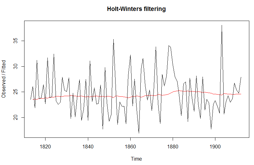
The plot shows the original time series in black, and the forecasts as a red line.

As a measure of the accuracy of the forecasts, calculate the sum of squared errors. The sum-of squared-errors is stored in a named element of the list variable “datatimeseriesforecast” called “SSE”.

datatimeseriesforecast$SSE

R console output

 

It is common in simple exponential smoothing to use the first value in the time series as the initial value for the level.

HoltWinters(datatimeseries,beta=FALSE, gamma=FALSE, l.start=23.56)

HoltWinters() just makes forecasts for the time period covered by the original data. We can make forecasts for further time points by using the “forecast.HoltWinters()” function in the R “forecast” package.

To use the forecast.HoltWinters() function, we first need to install the “forecast” R package (for instructions on how to install an R package, see How to install an R package).

Lets install forecast R package

install.package("forecast")

When using the forecast.HoltWinters() function, as its first argument (input), you pass it the predictive model that you have already fitted using the HoltWinters() function. For example, in the case of the rainfall time series, we stored the predictive model made using HoltWinters() in the variable “datatimeseriesforecast”. You specify how many further time points you want to make forecasts for by using the “h” parameter in forecast.HoltWinters(). For example, to make a forecast of rainfall for the years 1913-1920 (8 more years) using forecast.HoltWinters(). See below

datatimeseriesforecastpackage<-forecast.HoltWinters(datatimeseriesforecast h=8)
datatimeseriesforecastpackage

R console output

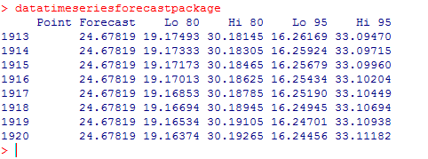
The forecast.HoltWinters() function gives you the forecast for a year, a 80% prediction interval for the forecast, and a 95% prediction interval for the forecast. For example, the forecasted rainfall for 1920 is about 24.68 inches, with a 95% prediction interval of (16.24, 33.11).

To plot the predictions made by forecast.HoltWinters(), we can use the “plot.forecast()” function:

plot.forecast(datatimeseriesforecastpackage)

Here the rain forecast for the time interval of 1913-1920 plotted as a blue line, the 80% prediction area is plotted in dark color shaded area and 95% plotted as light color shaded area.

The ‘forecast errors’ are calculated as the observed values minus predicted values, for each time point. We can only calculate the forecast error, for the time period covered in our original time series data, which 1813-1912. As mentioned above, one measure of the accuracy of the predictive model is the sum-of-squared errors (SSE) for the in-sample forecast errors.

The in-sample forecast errors are stored in the named element “residuals” of the list variable returned by forecast. HoltWinters().

If there are correlations between forecast errors for successive predictions, it is likely that the simple exponential smoothing forecasts could be improved upon by another forecasting technique.

Lets check, we can obtain a correlogram of the in-sample forecast errors for lags 1-20. We can calculate a correlogram of the forecast errors using the “acf()” function in R. To specify the maximum lag that we want to look at, we use the “lag.max” parameter in acf().

acf(datatimeseriesforecastpackage$resuduals, lag.max=20)

if you get an na.fail.default(ts(x)), then use this command to omit NA’S

acf(datatimeseriesforecastpackage$resuduals, lag.max=20,na.action=na.pass)

Here is the plot

You can see from the sample correlogram that the autocorrelation at lag 3 is just touching the significance bounds. To test whether there is significant evidence for non-zero correlations at lags 1-20, we can carry out a Ljung-Box test.

This can be done in R using Box.test() function

To test, if there is any non-zero autocorrelation in between lag(1-20)

box.test(datatimeseriesforecast$residual, lag=20, type= LjungBox)

Here is the R output

Here the Ljung-Box test statistic is 17.4, and the p-value is 0.6, so there is little evidence of non-zero autocorrelations in the in-sample forecast errors at lags 1-20.
To be sure that the predictive model cannot be improved upon, it is also a good idea to check whether the forecast errors are normally distributed with mean zero and constant variance. To check whether the forecast errors have constant variance, we can make a time plot of the in-sample forecast errors:

plot.ts(datatimeseriesforecastpackage$residuals)

here is the plot

The plot shows that the in-sample forecast errors seem to have roughly constant variance over time, although the size of the fluctuations in the start of the time series (1820-1830) may be slightly less than that at later dates (eg.1840-1850).

Forecasting time series of rainfall is done. If you have any doubts please share your views in comment section or shoot me an email irrfankhann29@gmail.com.